Table of Contents

Here is my first kernel along with my very first attempt at the Titanic challenge (newbie still learning …). The goal is to achieve a binary classification in order to predict whether a passenger survived the Titanic sinking (variable ‘Survived’). Read on Kaggle.

Data import & wrangling #

Titanic training dataset overview

PassengerId	Survived	Pclass	Name	Sex	Age	SibSp	Parch	Ticket	Fare	Cabin	Embarked
1	0	3	Braund, Mr. Owen Harris	male	22	1	0	A/5 21171	7.2500	NA	S
2	1	1	Cumings, Mrs. John Bradley (Florence Briggs Thayer)	female	38	1	0	PC 17599	71.2833	C85	C
3	1	3	Heikkinen, Miss. Laina	female	26	0	0	STON/O2. 3101282	7.9250	NA	S
4	1	1	Futrelle, Mrs. Jacques Heath (Lily May Peel)	female	35	1	0	113803	53.1000	C123	S
5	0	3	Allen, Mr. William Henry	male	35	0	0	373450	8.0500	NA	S
6	0	3	Moran, Mr. James	male	NA	0	0	330877	8.4583	NA	Q
7	0	1	McCarthy, Mr. Timothy J	male	54	0	0	17463	51.8625	E46	S
8	0	3	Palsson, Master. Gosta Leonard	male	2	3	1	349909	21.0750	NA	S
9	1	3	Johnson, Mrs. Oscar W (Elisabeth Vilhelmina Berg)	female	27	0	2	347742	11.1333	NA	S
10	1	2	Nasser, Mrs. Nicholas (Adele Achem)	female	14	1	0	237736	30.0708	NA	C

At first sight

Some variables are qualitative: Pclass (1, 2 or 3), Sex (male or female) and Embarked (C, Q or S).
Some variables are quantitative: Age, SibSp, Parch and Fare.
Some variables contain missing values.
Within the ‘Name’ variable, the passenger’s title (Miss., Master., Captain.) could be useful information for the predictions.

Missing value rate within variables

map_dbl(titanicTrainingDataset, function(x) mean(is.na(x)))

## PassengerId    Survived      Pclass        Name         Sex         Age
## 0.000000000 0.000000000 0.000000000 0.000000000 0.000000000 0.198653199
##       SibSp       Parch      Ticket        Fare       Cabin    Embarked
## 0.000000000 0.000000000 0.000000000 0.000000000 0.771043771 0.002244669

The Age variable contains 19.86% missing values and the Cabin one contains 77.1%. I will not use the Cabin variable as there are too many missing values.

Import the Titanic training dataset with proper col types for categorical variables

titanicTrainingDataset <- read_csv(
  trainFile,
  col_types = cols(
    Survived = col_factor(0:1),
    Pclass = col_factor(1:3),
    Sex = col_factor(c("male", "female")),
    Embarked = col_factor(c("C", "Q", "S"))
  )
) %>%
  filter(!is.na(Embarked)) %>%
  mutate(Age = ifelse(is.na(Age), median(Age, na.rm = T), Age))

I filled the blank values for the Age variable with the median age and excluded the rows that have no value for ‘Embarked’.

Extract the passengers’ titles from their names into a new dedicated variable

titanicTrainingDataset <- titanicTrainingDataset %>%
  mutate(Title = as.factor(str_extract(Name, regex("([a-z]+\\.)", ignore_case = T))))

levels(titanicTrainingDataset$Title)

##  [1] "Capt."     "Col."      "Countess." "Don."      "Dr."
##  [6] "Jonkheer." "Lady."     "Major."    "Master."   "Miss."
## [11] "Mlle."     "Mme."      "Mr."       "Mrs."      "Ms."
## [16] "Rev."      "Sir."

17 distinct titles have been extracted from the ‘Name’ variable.

Exploratory Data Analysis #

summary(titanicTrainingDataset)

##   PassengerId  Survived Pclass      Name               Sex
##  Min.   :  1   0:549    1:214   Length:889         male  :577
##  1st Qu.:224   1:340    2:184   Class :character   female:312
##  Median :446            3:491   Mode  :character
##  Mean   :446
##  3rd Qu.:668
##  Max.   :891
##
##       Age            SibSp            Parch           Ticket
##  Min.   : 0.42   Min.   :0.0000   Min.   :0.0000   Length:889
##  1st Qu.:22.00   1st Qu.:0.0000   1st Qu.:0.0000   Class :character
##  Median :28.00   Median :0.0000   Median :0.0000   Mode  :character
##  Mean   :29.32   Mean   :0.5242   Mean   :0.3825
##  3rd Qu.:35.00   3rd Qu.:1.0000   3rd Qu.:0.0000
##  Max.   :80.00   Max.   :8.0000   Max.   :6.0000
##
##       Fare            Cabin           Embarked     Title
##  Min.   :  0.000   Length:889         C:168    Mr.    :517
##  1st Qu.:  7.896   Class :character   Q: 77    Miss.  :181
##  Median : 14.454   Mode  :character   S:644    Mrs.   :124
##  Mean   : 32.097                               Master.: 40
##  3rd Qu.: 31.000                               Dr.    :  7
##  Max.   :512.329                               Rev.   :  6
##                                                (Other): 14

titanicTrainingDataset %>%
  ggplot(aes(x = Survived)) +
  geom_bar()

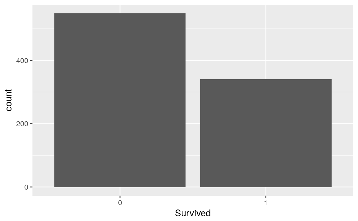
The following function will help me to visualize the response ‘Survived’ against each qualitative or quantitative potential predictor.

analysePredictorResponse <- function(data, predictor, response) {
  if (is.factor(data[[predictor]])) {
      ggplot(mapping = aes(data[[predictor]], fill = data[[response]])) +
        geom_bar() +
        labs(title = paste(predictor, "vs", response), x = predictor, fill = response)
  } else {
    chart1 <- ggplot(mapping = aes(data[[response]], data[[predictor]])) +
      geom_boxplot() +
      labs(title = paste(predictor, "vs", response), x = response, y = predictor)

    chart2 <- ggplot(mapping = aes(x = data[[predictor]], , y = ..density.., colour = data[[response]])) +
      geom_freqpoly(position = "dodge") +
      labs(title = paste(predictor, "vs", response), colour = response, x = predictor)

    grid.arrange(chart1, chart2)
  }
}

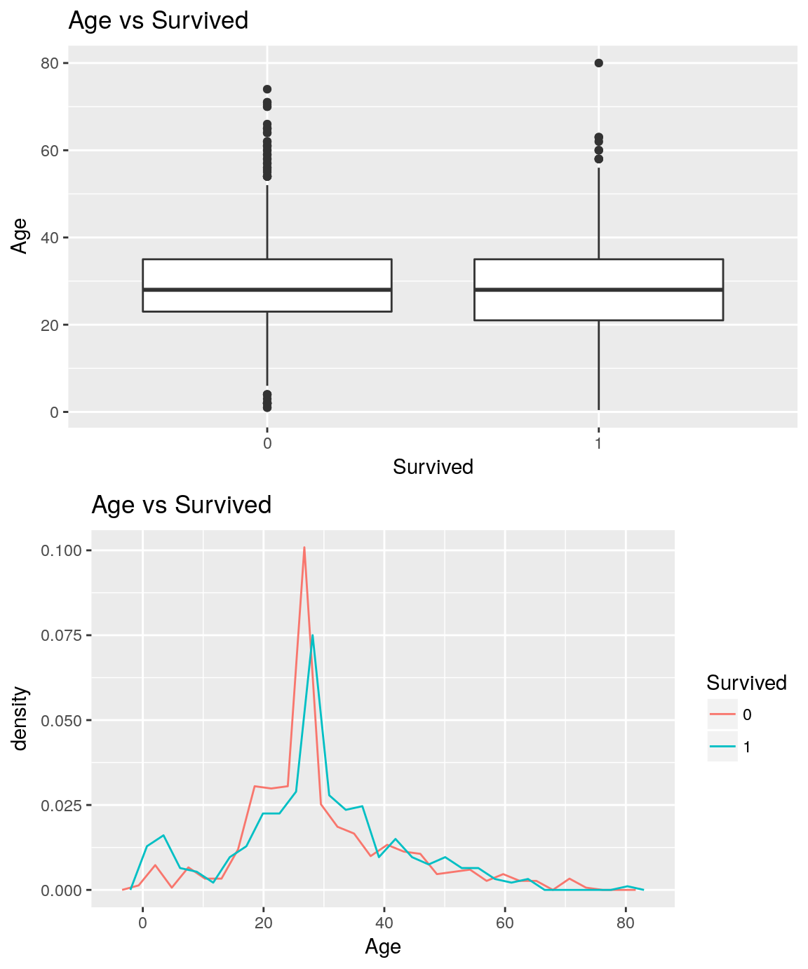
Age vs Survived

analysePredictorResponse(titanicTrainingDataset, 'Age', 'Survived')

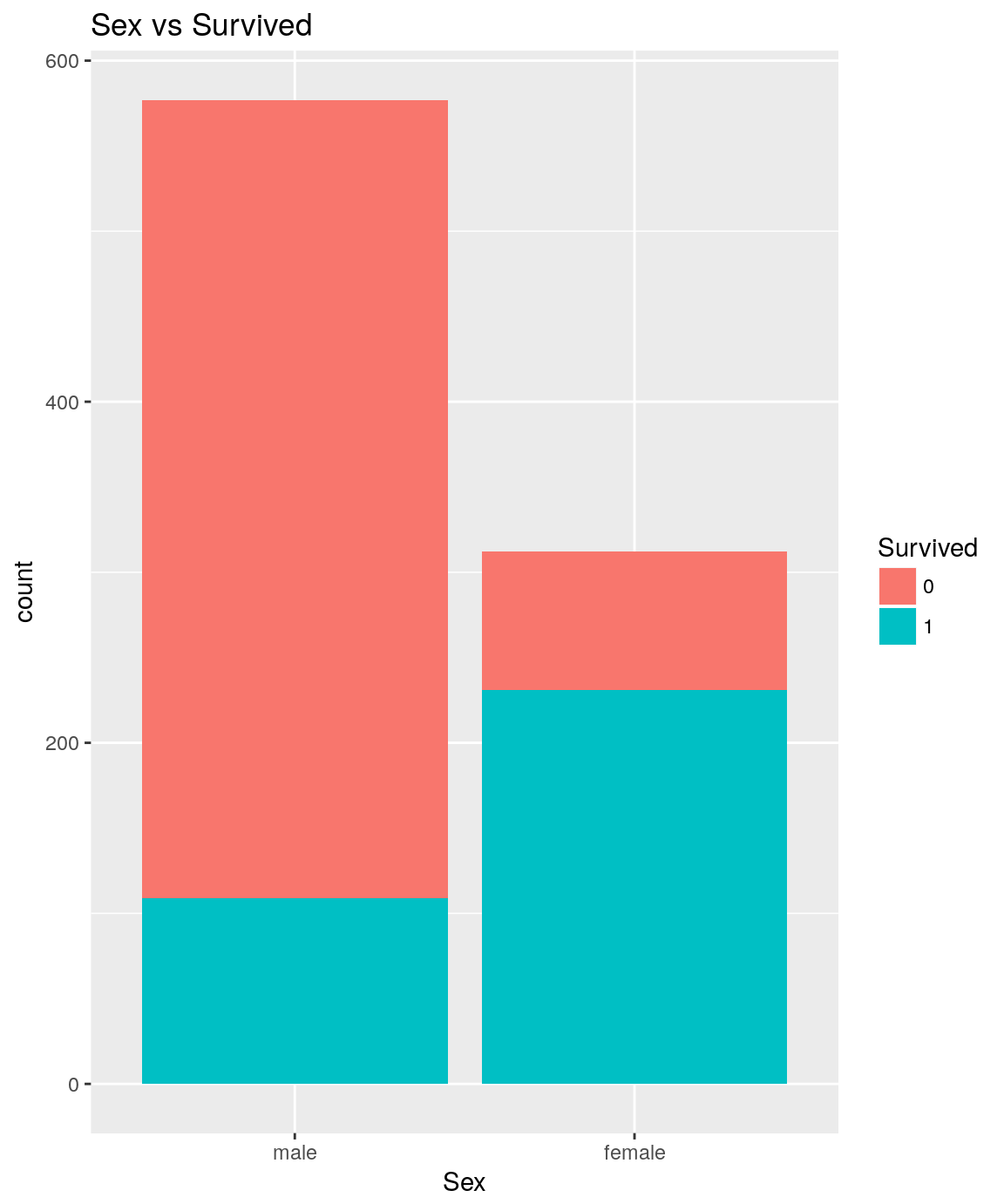
Sex vs Survived

analysePredictorResponse(titanicTrainingDataset, 'Sex', 'Survived')

titanicTrainingDataset %>%
  group_by(Sex) %>%
  summarize(SurvivedRatio = mean(Survived == 1))

## # A tibble: 2 x 2
##   Sex    SurvivedRatio
##   <fct>          <dbl>
## 1 male           0.189
## 2 female         0.740

It seems obvious that females have significantly more chance of surviving than males.

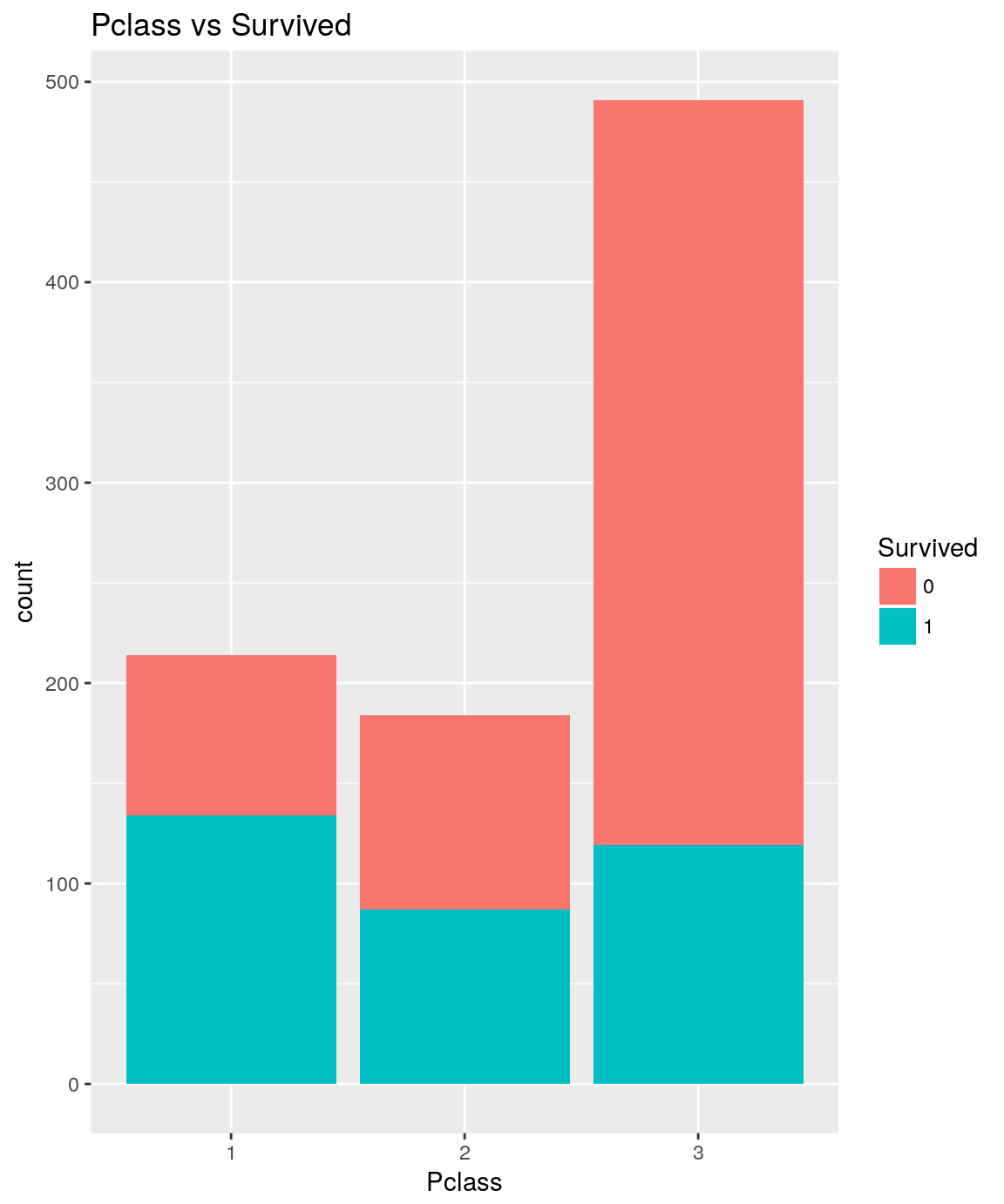
Pclass vs Survived

analysePredictorResponse(titanicTrainingDataset, 'Pclass', 'Survived')

titanicTrainingDataset %>%
  group_by(Pclass) %>%
  summarize(SurvivedRatio = mean(Survived == 1))

## # A tibble: 3 x 2
##   Pclass SurvivedRatio
##   <fct>          <dbl>
## 1 1              0.626
## 2 2              0.473
## 3 3              0.242

The wealthier the class the passenger belongs to, the higher their likelihood of surviving.

SibSp vs Survived

analysePredictorResponse(titanicTrainingDataset, 'SibSp', 'Survived')

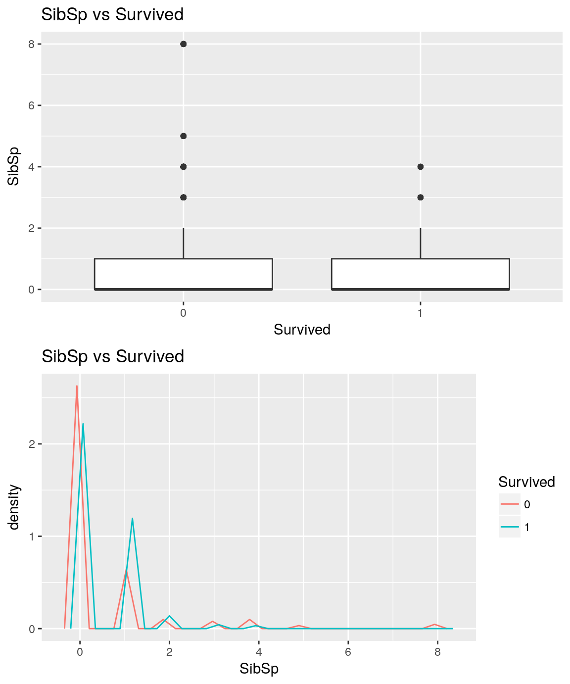
Those who have no sibling seem to have a higher chance of dying than those who have one sibling on board.

Parch vs Survived

analysePredictorResponse(titanicTrainingDataset, 'Parch', 'Survived')

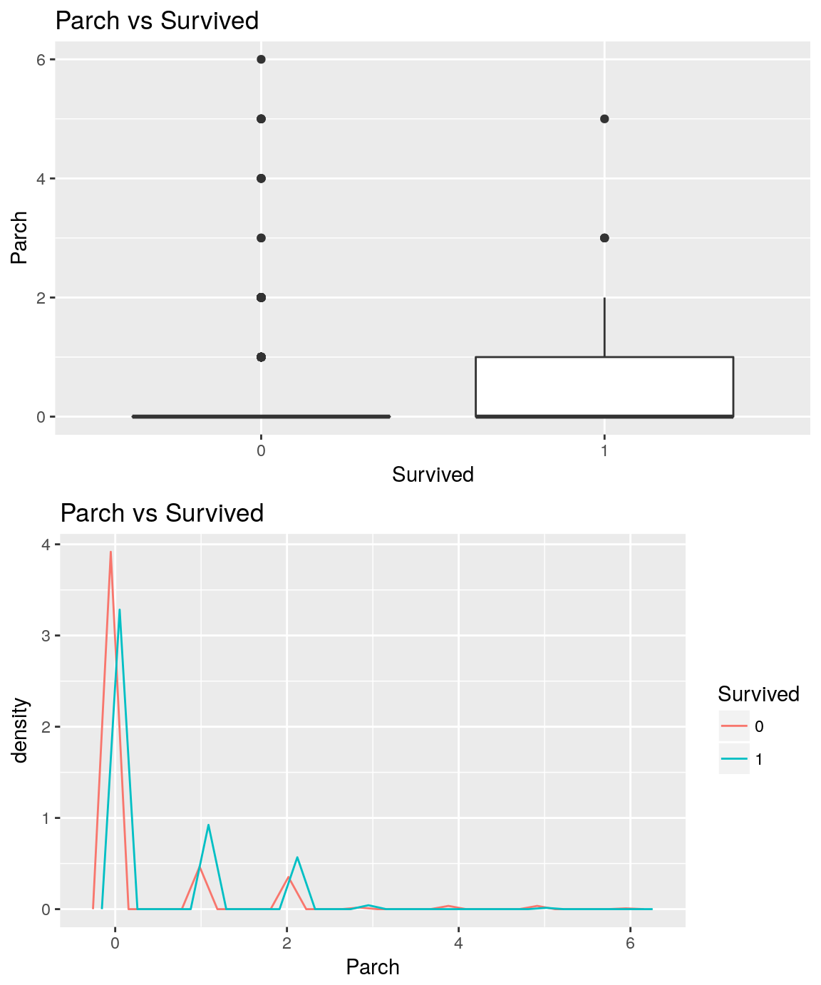
Similarly to SibSp, those who have no parents or children on board seem to have a higher chance of dying than those who have one parent or one child.

Fare vs Survived

analysePredictorResponse(titanicTrainingDataset, 'Fare', 'Survived')

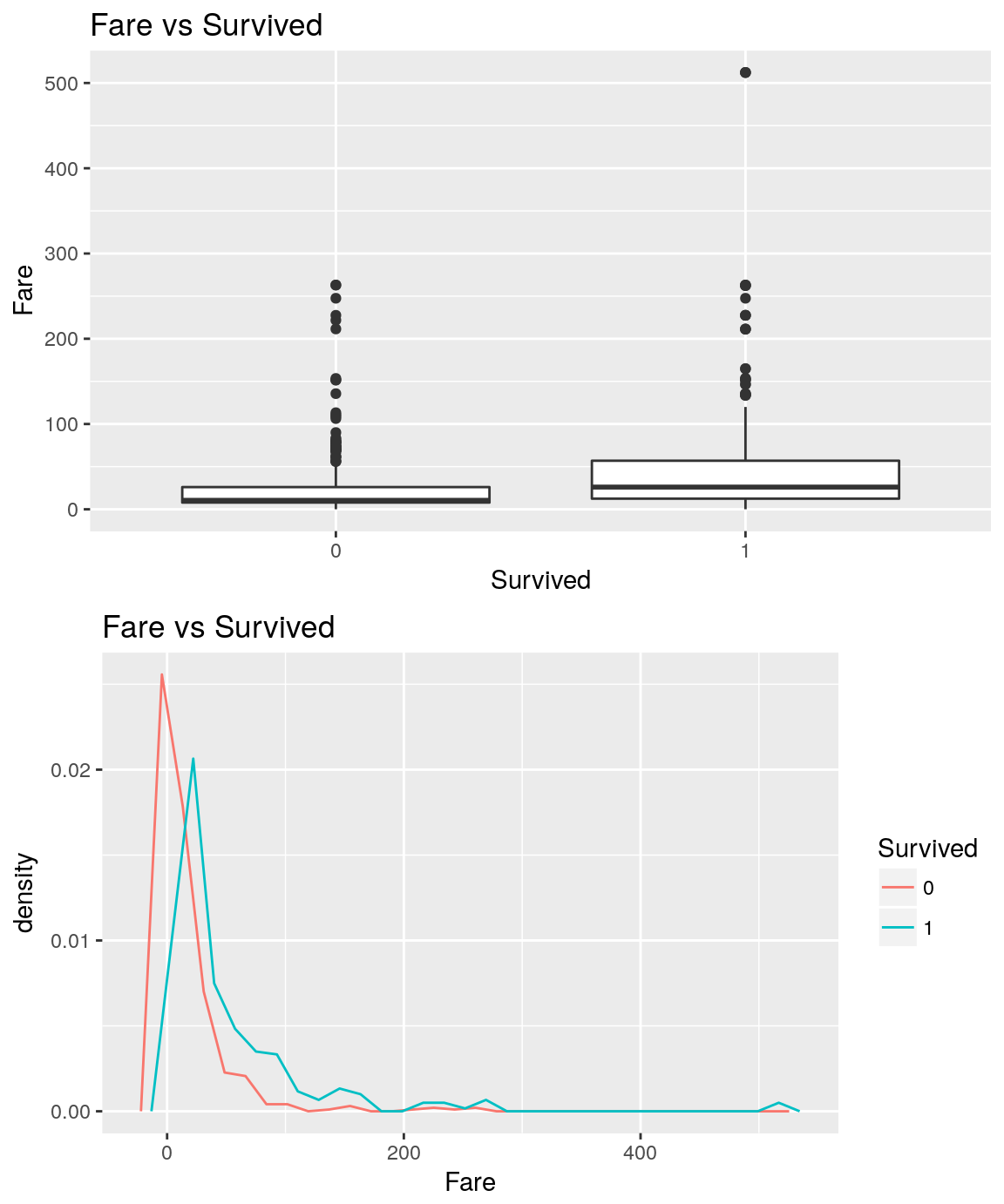
On average, the higher the fare, the higher the likelihood of surviving seems to be.

Embarked vs Survived

analysePredictorResponse(titanicTrainingDataset, 'Embarked', 'Survived')

titanicTrainingDataset %>%
  group_by(Embarked) %>%
  summarize(SurvivedRatio = mean(Survived == 1))

## # A tibble: 3 x 2
##   Embarked SurvivedRatio
##   <fct>            <dbl>
## 1 C                0.554
## 2 Q                0.390
## 3 S                0.337

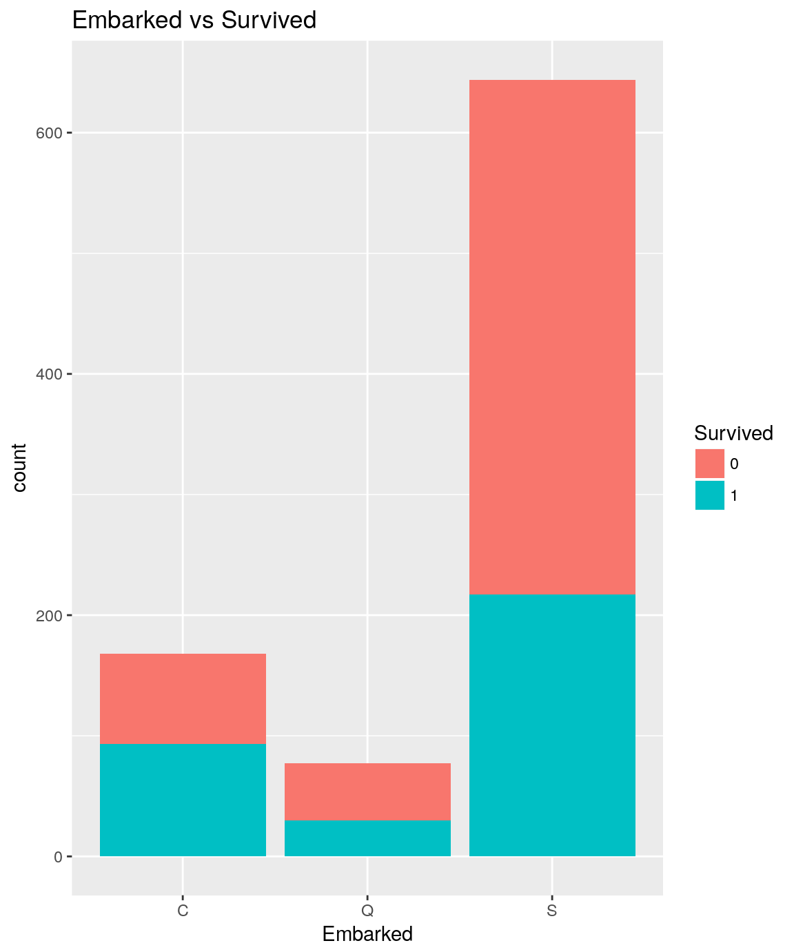
It seems there are some significant differences regarding the Survived rate depending on the port of embarkation. Port C leads to a 55.36% survival rate whereas port S leads to only 33.69%.

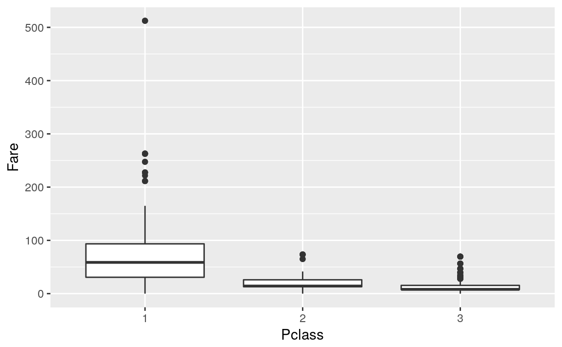
Pclass vs Fare

titanicTrainingDataset %>%
  ggplot(mapping = aes(Pclass, Fare)) +
  geom_boxplot()

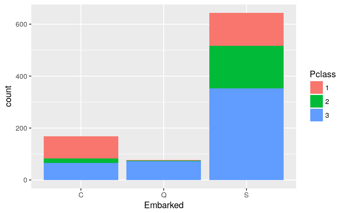
Embarked vs Pclass

titanicTrainingDataset %>%
  ggplot(mapping = aes(Embarked, fill = Pclass)) +
  geom_bar()

What about the variable Title that I have extracted from the names?

titanicTrainingDataset %>%
  group_by(Title) %>%
  summarize(SurvivedRatio = mean(Survived == 1)) %>%
  arrange(SurvivedRatio) %>%
  mutate(Title = factor(Title, levels = Title)) %>%
  ggplot(aes(x = Title, y = SurvivedRatio)) +
  geom_col() +
  coord_flip()

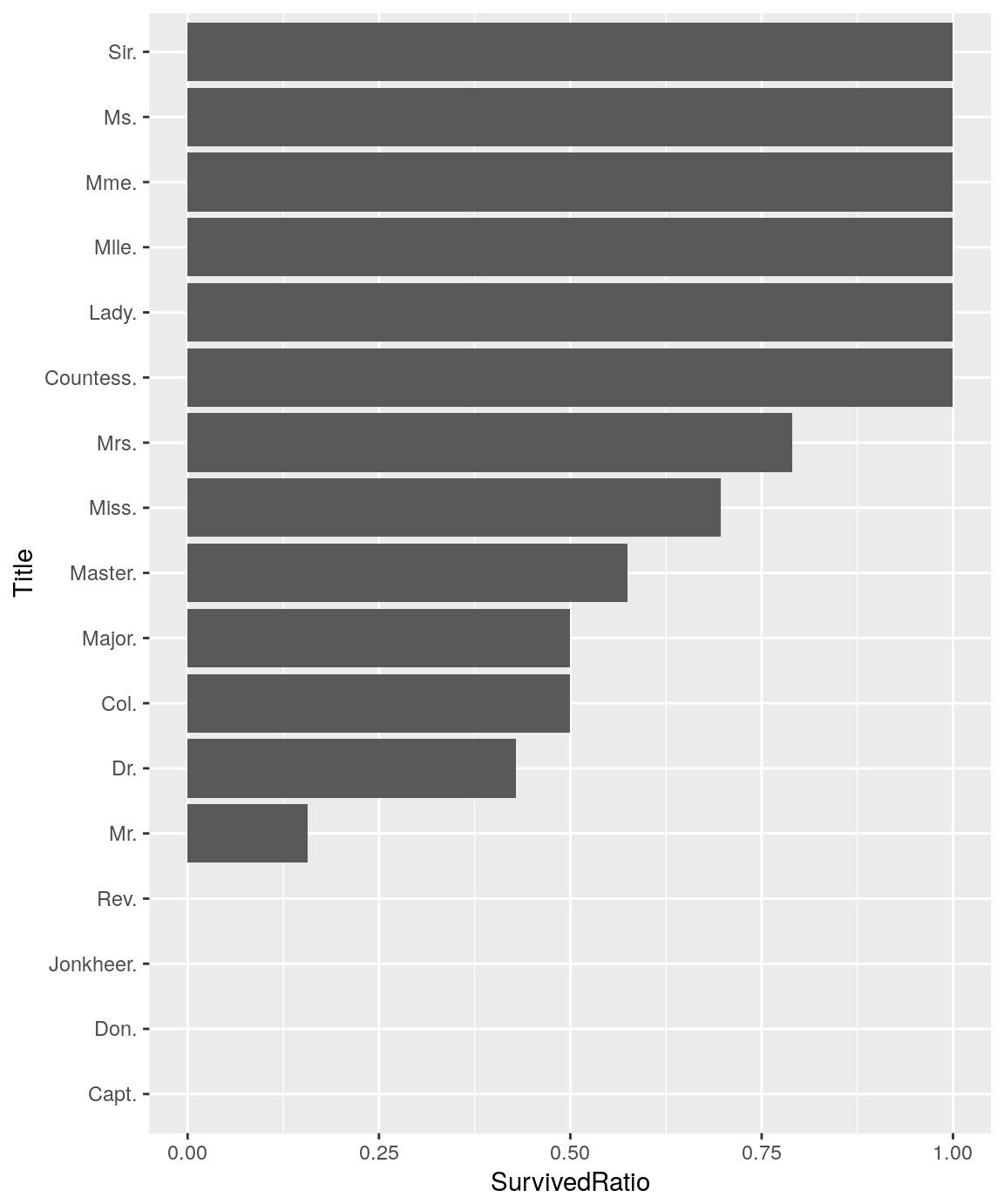
The passengers’ title seems to provide interesting information for predicting the survivors. It seems we can refine this variable in order to reduce the number of levels. I added a new categorical variable ‘RefinedTitle’ that splits the passengers’ titles into 3 relevant levels:

titanicTrainingDataset <- titanicTrainingDataset %>% mutate(
  RefinedTitle = factor(ifelse(Title %in% c('Capt.', 'Don', 'Jonkheer.', 'Rev.', 'Mr.'), 1,
    ifelse(Title %in% c('Col.', 'Dr.', 'Major.', 'Master.'), 2, 3
    )
  ))
)

Modeling #

Logistic regression #

Here is a first attempt at modeling on the training dataset with most of the candidate predictors:

model <- glm(Survived ~ RefinedTitle + Pclass + SibSp + Embarked + Age + Sex + Parch, data = titanicTrainingDataset %>% filter(!is.na(Age)), family = binomial)
summary(model)

##
## Call:
## glm(formula = Survived ~ RefinedTitle + Pclass + SibSp + Embarked +
##     Age + Sex + Parch, family = binomial, data = titanicTrainingDataset %>%
##     filter(!is.na(Age)))
##
## Deviance Residuals:
##     Min       1Q   Median       3Q      Max
## -2.3632  -0.5951  -0.3917   0.5812   2.5346
##
## Coefficients:
##                Estimate Std. Error z value Pr(>|z|)
## (Intercept)    0.930213   0.393458   2.364 0.018069 *
## RefinedTitle2  2.556167   0.426595   5.992 2.07e-09 ***
## RefinedTitle3  0.473372   1.439032   0.329 0.742192
## Pclass2       -1.032744   0.282392  -3.657 0.000255 ***
## Pclass3       -2.163955   0.262944  -8.230  < 2e-16 ***
## SibSp         -0.452722   0.114388  -3.958 7.56e-05 ***
## EmbarkedQ     -0.274539   0.392170  -0.700 0.483895
## EmbarkedS     -0.484066   0.244469  -1.980 0.047696 *
## Age           -0.027045   0.008209  -3.294 0.000986 ***
## Sexfemale      2.672175   1.448318   1.845 0.065035 .
## Parch         -0.189686   0.122467  -1.549 0.121413
## ---
## Signif. codes:  0 '***' 0.001 '**' 0.01 '*' 0.05 '.' 0.1 ' ' 1
##
## (Dispersion parameter for binomial family taken to be 1)
##
##     Null deviance: 1182.8  on 888  degrees of freedom
## Residual deviance:  745.7  on 878  degrees of freedom
## AIC: 767.7
##
## Number of Fisher Scoring iterations: 5

Parch and Embarked don’t seem to be relevant according to the P-value associated with the Z-statistic. Also, Sex seems to be confounded with RefinedTitle for predicting ‘Survived’. Here is a refined model without the Parch, Embarked and Sex variables:

model <- glm(Survived ~ RefinedTitle + Pclass + SibSp + Age, data = titanicTrainingDataset, family = binomial)
summary(model)

##
## Call:
## glm(formula = Survived ~ RefinedTitle + Pclass + SibSp + Age,
##     family = binomial, data = titanicTrainingDataset)
##
## Deviance Residuals:
##     Min       1Q   Median       3Q      Max
## -2.5200  -0.5798  -0.3934   0.5919   2.6299
##
## Coefficients:
##                Estimate Std. Error z value Pr(>|z|)
## (Intercept)    0.646841   0.368287   1.756 0.079029 .
## RefinedTitle2  2.484859   0.415967   5.974 2.32e-09 ***
## RefinedTitle3  3.066697   0.207374  14.788  < 2e-16 ***
## Pclass2       -1.153534   0.271979  -4.241 2.22e-05 ***
## Pclass3       -2.227890   0.250689  -8.887  < 2e-16 ***
## SibSp         -0.524237   0.110349  -4.751 2.03e-06 ***
## Age           -0.028450   0.008128  -3.500 0.000465 ***
## ---
## Signif. codes:  0 '***' 0.001 '**' 0.01 '*' 0.05 '.' 0.1 ' ' 1
##
## (Dispersion parameter for binomial family taken to be 1)
##
##     Null deviance: 1182.82  on 888  degrees of freedom
## Residual deviance:  754.59  on 882  degrees of freedom
## AIC: 768.59
##
## Number of Fisher Scoring iterations: 5

All the coefficient estimates for predictors are now statistically significant according to their P-Values.

Estimate the test error rate of the logistic regression with LOOCV #

Here is a “leave-one-out” cross validation performed over several decision boundary values (from 0.1 to 0.9) in order to find the value that minimizes the simulated test error rate with the training dataset. For each value, it will display the estimated error rate along with the confusion matrix.

for (j in seq(.1, .9, .1)) {
  predictions <- rep(0, nrow(titanicTrainingDataset))
  for (i in 1:nrow(titanicTrainingDataset)) {
    model <- glm(Survived ~ RefinedTitle + Pclass + SibSp + Age, data = titanicTrainingDataset, family = binomial, subset = -i)
    predictions[i] <- predict(model, titanicTrainingDataset[i,], type = "response") > j
  }

  print(paste("Decision boundary value :", j))
  print(table(predictions, titanicTrainingDataset$Survived))
  print(mean(predictions != titanicTrainingDataset$Survived))
}

## [1] "Decision boundary value : 0.1"
##
## predictions   0   1
##           0 250  33
##           1 299 307
## [1] 0.3734533
## [1] "Decision boundary value : 0.2"
##
## predictions   0   1
##           0 346  44
##           1 203 296
## [1] 0.2778403
## [1] "Decision boundary value : 0.3"
##
## predictions   0   1
##           0 423  57
##           1 126 283
## [1] 0.2058493
## [1] "Decision boundary value : 0.4"
##
## predictions   0   1
##           0 443  68
##           1 106 272
## [1] 0.1957255
## [1] "Decision boundary value : 0.5"
##
## predictions   0   1
##           0 482  92
##           1  67 248
## [1] 0.1788526
## [1] "Decision boundary value : 0.6"
##
## predictions   0   1
##           0 501 110
##           1  48 230
## [1] 0.1777278
## [1] "Decision boundary value : 0.7"
##
## predictions   0   1
##           0 523 152
##           1  26 188
## [1] 0.200225
## [1] "Decision boundary value : 0.8"
##
## predictions   0   1
##           0 538 198
##           1  11 142
## [1] 0.2350956
## [1] "Decision boundary value : 0.9"
##
## predictions   0   1
##           0 544 276
##           1   5  64
## [1] 0.3160855

The estimated test error rate seems to be minimized with a decision boundary value of 0.6, resulting in a test error rate of 17.77%.

Use the logistic regression model to predict the Survived variable with the test dataset #

model <- glm(Survived ~ RefinedTitle + Pclass + SibSp + Age, data = titanicTrainingDataset, family = binomial)

titanicTestDataset <- read_csv(
  testFile,
  col_types = cols(
    Pclass = col_factor(1:3),
    Sex = col_factor(c("male", "female")),
    Embarked = col_factor(c("C", "Q", "S"))
  )
) %>%
  mutate(Title = as.factor(str_extract(Name, regex("([a-z]+\\.)", ignore_case = T)))) %>%
  mutate(
    RefinedTitle = factor(ifelse(Title %in% c('Capt.', 'Don', 'Jonkheer.', 'Rev.', 'Mr.'), 1,
      ifelse(Title %in% c('Col.', 'Dr.', 'Major.', 'Master.'), 2, 3
      )
    ))
  ) %>%
  mutate(Age = ifelse(is.na(Age), median(Age, na.rm = T), Age))

predictions <- predict(model, titanicTestDataset, type = "response") > .6

tibble(PassengerId = titanicTestDataset$PassengerId, Survived = as.integer(predictions)) %>%
  write_csv('predictions-logistic-regression.csv')

The Kaggle score is 77.5% with this model.

Quadratic Discriminant Analysis #

model <- qda(Survived ~ RefinedTitle + Pclass + SibSp + Age, data = titanicTrainingDataset, family = binomial)
model

## Call:
## qda(Survived ~ RefinedTitle + Pclass + SibSp + Age, data = titanicTrainingDataset,
##     family = binomial)
##
## Prior probabilities of groups:
##         0         1
## 0.6175478 0.3824522
##
## Group means:
##   RefinedTitle2 RefinedTitle3   Pclass2   Pclass3     SibSp      Age
## 0    0.04189435     0.1493625 0.1766849 0.6775956 0.5537341 30.02823
## 1    0.08235294     0.6794118 0.2558824 0.3500000 0.4764706 28.16374

LOOCV on the QDA model #

predictions <- factor(rep(0, nrow(titanicTrainingDataset)), levels = 0:1)
for (i in 1:nrow(titanicTrainingDataset)) {
  model <- qda(Survived ~ RefinedTitle + Pclass + SibSp + Age, data = titanicTrainingDataset, subset = -i)
  predictions[i] <- predict(model, titanicTrainingDataset[i,])$class
}

table(predictions, titanicTrainingDataset$Survived)

##
## predictions   0   1
##           0 451  78
##           1  98 262

mean(predictions != titanicTrainingDataset$Survived)

## [1] 0.1979753

The estimated test error rate is 19.79% with the Quadratic Discriminant Analysis model.

Use the QDA model to predict the Survived variable with the test dataset from Kaggle #

model <- qda(Survived ~ RefinedTitle + Pclass + SibSp + Age, data = titanicTrainingDataset)
predictions <- predict(model, titanicTestDataset)$class

tibble(PassengerId = titanicTestDataset$PassengerId, Survived = predictions) %>%
  write_csv('predictions-qda.csv')

The Kaggle score is 77.5%, almost like the logistic regression.

K-nearest neighbors #

Let’s keep the same set of predictors that seem to be relevant to predict the response, and use the KNN algorithm with them. First, I evaluate the best K value with a Validation Set approach, by splitting the training dataset into a training and a test dataset:

set.seed(1)
titanicTrainingDatasetKnn <- titanicTrainingDataset
titanicTrainingDatasetKnn$RefinedTitle = as.integer(titanicTrainingDatasetKnn$RefinedTitle)
titanicTrainingDatasetKnn$Pclass = as.integer(titanicTrainingDatasetKnn$Pclass)

testSampleSize <- 150
isTest <- sample(nrow(titanicTrainingDataset), testSampleSize)

knnTrainDataset <- titanicTrainingDatasetKnn[-isTest,] %>%
  subset(select = c(RefinedTitle, Pclass, SibSp, Age)) %>%
  scale()

knnTestDataset <- titanicTrainingDatasetKnn[isTest,] %>%
  subset(select = c(RefinedTitle, Pclass, SibSp, Age)) %>%
  scale()

cl <- titanicTrainingDatasetKnn[-isTest,]$Survived

errorsRate <- rep(0, testSampleSize)
for (k in 1:testSampleSize) {
  predictions <- knn(knnTrainDataset, knnTestDataset, cl, k)
  errorsRate[k] = mean(predictions != titanicTrainingDatasetKnn[isTest,]$Survived)
}

tibble(k = 1:testSampleSize, errorsRate = errorsRate) %>%
  ggplot(aes(x = k, y = errorsRate)) +
  geom_path()

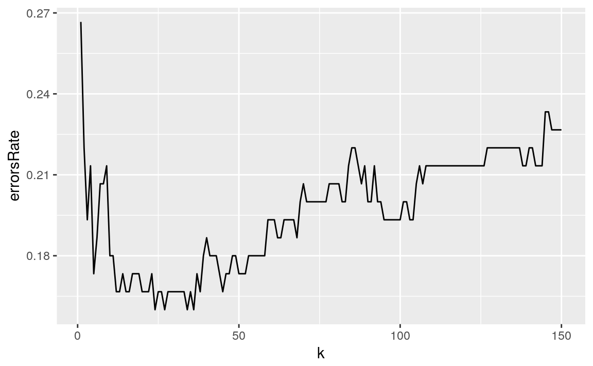
I choose k = 35 to minimize the test error rate.

Use KNN (K = 35) to predict the response with the test dataset #

titanicTestDatasetKnn <- titanicTestDataset %>%
  mutate(RefinedTitle = as.integer(RefinedTitle)) %>%
  mutate(Pclass = as.integer(Pclass))

knnTrainDataset <- titanicTrainingDatasetKnn %>%
  subset(select = c(RefinedTitle, Pclass, SibSp, Age)) %>%
  scale()

knnTestDataset <- titanicTestDatasetKnn %>%
  subset(select = c(RefinedTitle, Pclass, SibSp, Age)) %>%
  scale()

cl <- titanicTrainingDatasetKnn$Survived

predictions <- knn(knnTrainDataset, knnTestDataset, cl, 35)

tibble(PassengerId = titanicTestDataset$PassengerId, Survived = predictions) %>%
  write_csv('predictions-knn.csv')

The Kaggle score is 78.94%.